Understanding Quantum State Evolution and Entanglement Dynamics with QuTiP

Quantum mechanics, a branch of physics that describes the behavior of matter and light at the atomic and subatomic levels, can seem incredibly complex. However, advancements in technology and software have made it easier to explore concepts like quantum state evolution, decoherence, and entanglement. One powerful tool for simulating these phenomena is QuTiP (Quantum Toolbox in Python). This blog post will guide you through the process of implementing quantum state evolution, decoherence, and entanglement dynamics using QuTiP, helping you understand these vital concepts in quantum mechanics.

What is QuTiP?

QuTiP is an open-source software library that allows researchers and enthusiasts to simulate the dynamics of quantum systems. It provides an intuitive and versatile framework to work with quantum states and operators, making it ideal for various applications in quantum computing, quantum optics, and quantum information theory. With QuTiP, users can easily create, manipulate, and visualize quantum states, enabling a deeper insight into complex quantum phenomena.

Quantum State Evolution

Quantum state evolution is a fundamental concept in quantum mechanics, describing how the state of a quantum system changes over time. This evolution is governed by the Schrödinger equation. In the context of QuTiP, we can model the evolution of a quantum state by defining the Hamiltonian of the system, which encapsulates the total energy of the quantum system.

Defining a Hamiltonian in QuTiP

To illustrate quantum state evolution, we will consider a simple two-level system (also known as a qubit). The Hamiltonian can be defined as follows:

python
from qutip import *

Define the Pauli-X operator

H = sigmax()

In this code snippet, we’ve defined a Hamiltonian using the Pauli-X operator. This operator represents a fundamental quantum gate that performs a bit-flip operation on the qubit.

Simulating Time Evolution

With the Hamiltonian defined, we can simulate the time evolution of the quantum state. Let’s assume our system starts in a specific state, denoted by ( |0\rangle ):

python

Initial state

psi0 = basis(2, 0) # |0> state

Time parameters

tlist = np.linspace(0, 10, 100) # Time points

Time evolution

result = mesolve(H, psi0, tlist, [], [sigmax(), sigmay(), sigmaz()])

In this code, we use the mesolve function to compute the dynamics of our system over a specified time range. The results provide valuable insights into how our initial quantum state evolves.

Understanding Decoherence

Decoherence is a phenomenon that arises when a quantum system interacts with its environment, leading to the loss of quantum coherence. This process is crucial for understanding why quantum states tend to lose their superposition and behave more classically over time.

Modeling Decoherence in QuTiP

In QuTiP, we can model decoherence by introducing environmental interactions. For example, we will use the Lindblad equation, which describes the dynamics of open quantum systems:

python
def decoherence_ops(gamma):
return [np.sqrt(gamma) * sigmax()]

Lindblad master equation

gamma = 0.1 # Decoherence rate
result = mesolve(H, psi0, tlist, decoherence_ops(gamma), [sigmax(), sigmay(), sigmaz()])

Here, we define a decoherence operator and use it in the mesolve function to simulate the effect of decoherence on our quantum state.

Exploring Entanglement Dynamics

Entanglement is one of the most fascinating aspects of quantum mechanics, where the quantum states of two or more particles become interconnected, such that the state of one particle instantly influences the state of another, regardless of the distance separating them.

Creating Entangled States

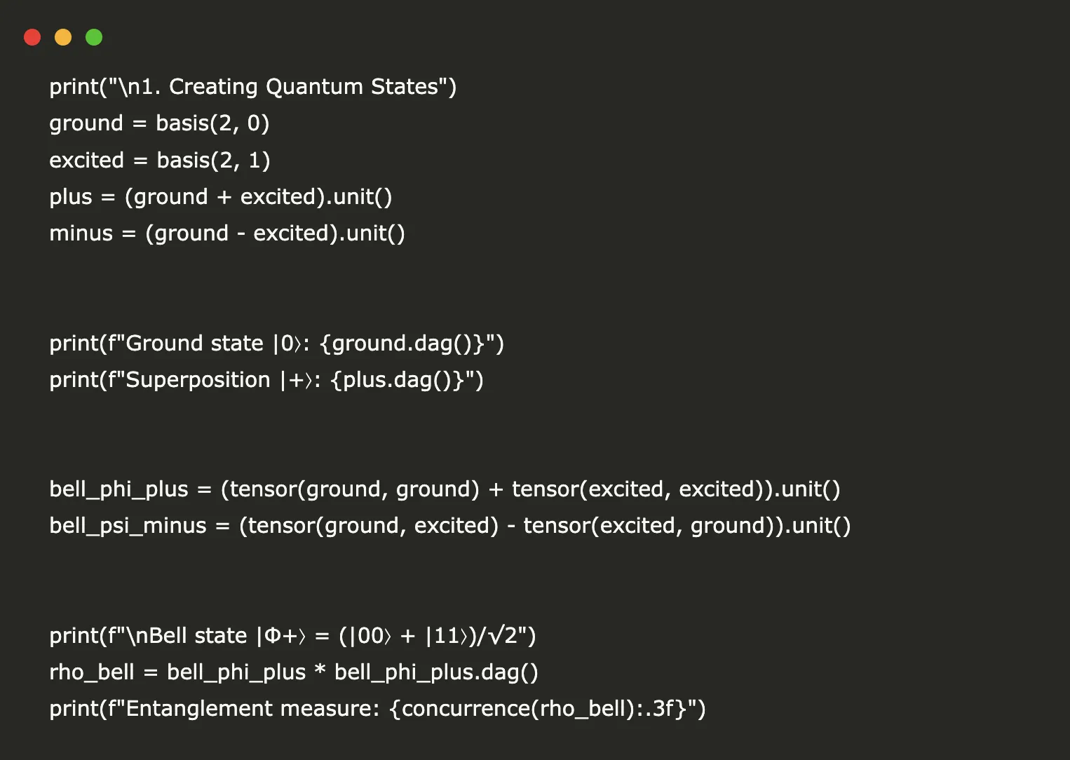
Let’s demonstrate how to create entangled states using QuTiP. We can utilize the Bell state, which is a common example of an entangled state:

python

Create Bell state |Φ+> = (|00> + |11>)/sqrt(2)

psi_entangled = (tensor(basis(2, 0), basis(2, 0)) + tensor(basis(2, 1), basis(2, 1))).unit()

In this snippet, we define the Bell state ( |Φ+\rangle ), which is a superposition of two basic states, showcasing quantum entanglement.

Dynamics of Entangled States

We can simulate the time evolution of our entangled state, observing how entanglement remains or is affected over time. This can also include considering decoherence:

python

Time evolution of the entangled state

result = mesolve(H, psi_entangled, tlist, decoherence_ops(gamma), [sigmax(), sigmay(), sigmaz()])

By monitoring the results, we can analyze how entangled states evolve and how they are affected by interactions with the environment.

Visualizing the Results

After completing the simulations, visualizing the results helps us understand the dynamics better. QuTiP provides built-in functions for plotting the results:

python
import matplotlib.pyplot as plt

plt.figure()
plt.plot(tlist, result.expect[0], label=’X Expectation’)
plt.plot(tlist, result.expect[1], label=’Y Expectation’)
plt.plot(tlist, result.expect[2], label=’Z Expectation’)
plt.xlabel(‘Time’)
plt.ylabel(‘Expectation Values’)
plt.legend()
plt.title(‘Quantum State Evolution’)
plt.show()

Visualizing the expectation values of different operators over time allows us to comprehend the evolution and decoherence of quantum states clearly, bringing our theoretical understanding to life.

Conclusion

The QuTiP library makes exploring the intricacies of quantum mechanics accessible and intuitive. By simulating quantum state evolution, decoherence, and entanglement dynamics, users can gain profound insights into how quantum systems behave. As quantum technology advances, understanding these fundamental concepts will be crucial for future developments in quantum computing and quantum information science. Whether you’re a seasoned researcher or a curious beginner, delving into these simulations can enhance your grasp of quantum mechanics like never before.